Intro Exercises
Practice exercises that reinforce the core image processing concepts from the previous guide - contrast manipulation via pixel-level math and binary thresholding for document analysis.
Prerequisites
import cv2
import numpy as np
import matplotlib.pyplot as plt
Exercise 1: Contrast Adjustment and Overflow
The goal of this exercise is to increase image contrast by multiplying every pixel value by a scalar, and to understand what happens when the result exceeds the 0-255 range that uint8 can represent.
Loading the Image
image = "Santorini.jpg"
img = cv2.imread(image, cv2.IMREAD_COLOR)
We load a color image of Santorini. OpenCV reads it in BGR format with pixel values in the [0, 255] range.
Building a Multiplier Matrix
matrix_ones = np.ones(img.shape, dtype="float64")
np.ones creates a matrix of the same shape as the image, filled with 1.0. We'll scale this matrix to create our contrast multipliers. Using float64 ensures we have enough precision for the multiplication before converting back to uint8.
Part A: Contrast Without Overflow Protection
img_higher1 = np.uint8(cv2.multiply(np.float64(img), matrix_ones * 1.1))
img_higher2 = np.uint8(cv2.multiply(np.float64(img), matrix_ones * 1.2))
Here we multiply every pixel by 1.1 and 1.2 to brighten and increase contrast. The critical issue is that np.uint8(...) wraps around on overflow: a pixel value of 260 does not become 255 - it wraps to 260 - 256 = 4, producing wild color artifacts.
plt.figure(figsize=[18, 5])
plt.subplot(131); plt.imshow(img[:, :, ::-1]);         plt.title("Original")
plt.subplot(132); plt.imshow(img_higher1[:, :, ::-1]); plt.title("Higher (1.1x)")
plt.subplot(133); plt.imshow(img_higher2[:, :, ::-1]); plt.title("Higher (1.2x)")
plt.show()
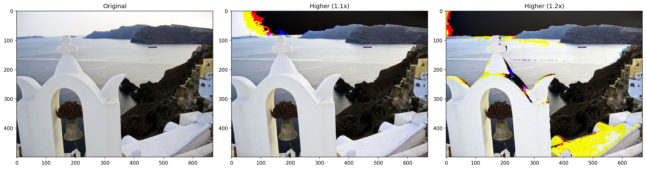
Notice the bright yellow and dark splotches in the sky and white walls. These are overflow artifacts - pixels that were near 255 wrapped around to small values, producing incorrect colors. The effect is more severe at 1.2x because more pixels exceed the 255 threshold.
Part B: Contrast With np.clip() Fix
img_higher1 = np.uint8(np.clip(cv2.multiply(np.float64(img), matrix_ones * 1.1), 0, 255))
img_higher2 = np.uint8(np.clip(cv2.multiply(np.float64(img), matrix_ones * 1.2), 0, 255))
The fix is np.clip(array, 0, 255), which clamps every value to the valid range before the uint8 conversion. A pixel value of 260 becomes 255 instead of wrapping to 4.
plt.figure(figsize=[18, 5])
plt.subplot(131); plt.imshow(img[:, :, ::-1]);         plt.title("Original")
plt.subplot(132); plt.imshow(img_higher1[:, :, ::-1]); plt.title("Higher (1.1x): clipped")
plt.subplot(133); plt.imshow(img_higher2[:, :, ::-1]); plt.title("Higher (1.2x): clipped")
plt.show()
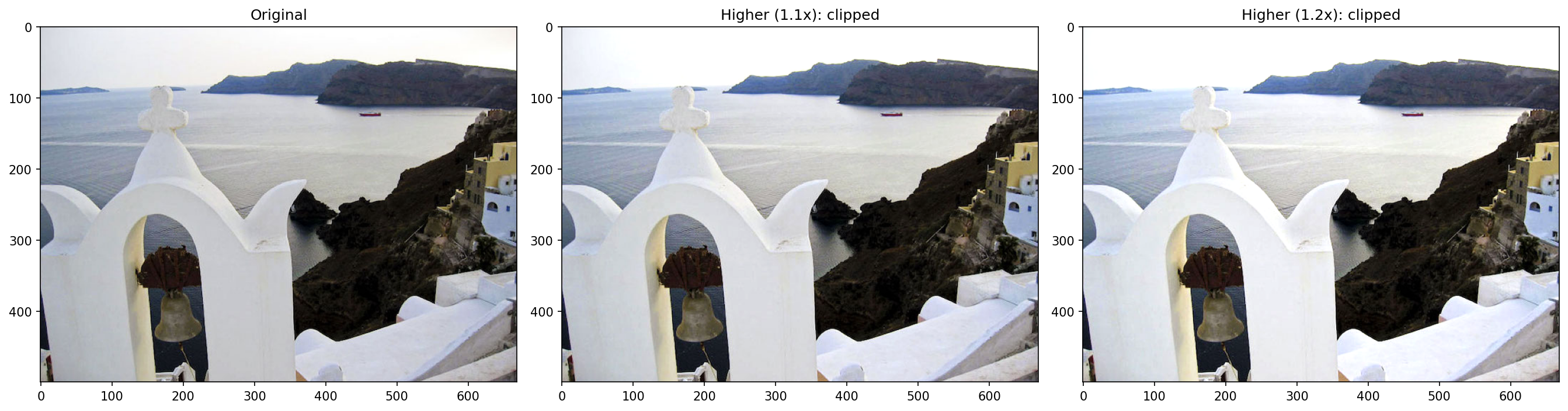
With clipping, both contrast-enhanced images look natural. Bright areas saturate to pure white rather than wrapping to dark values. This is a fundamental pattern in image processing: always clip or saturate after arithmetic operations on pixel values.
Key Takeaway
When performing arithmetic on images, pixel values can exceed the [0, 255] range. Converting directly to uint8 causes wraparound artifacts. Always use np.clip(result, 0, 255) before the type conversion to get correct results.
Exercise 2: Thresholding Sheet Music
This exercise applies global binary thresholding to a sheet music scan - a practical use case for document binarization where we want to separate ink (notes, staves, text) from the paper background.
Loading as Grayscale
img = cv2.imread('Sheet_Music_Test-1.jpg', cv2.IMREAD_GRAYSCALE)
We load the sheet music image directly in grayscale since we only care about intensity (dark ink vs. light paper). This gives us a single-channel image where each pixel is a value from 0 (black) to 255 (white).
Applying an Inverse Binary Threshold
retval, img_thresh = cv2.threshold(img, 130, 255, cv2.THRESH_BINARY_INV)
Let's break down the parameters:
img- the grayscale input image130- the threshold value. Pixels are classified based on whether they fall above or below this value255- the maximum value assigned to pixels that pass the threshold testcv2.THRESH_BINARY_INV- inverse binary mode: pixels below the threshold become255(white), and pixels above become0(black)
The inverse mode (_INV) is useful here because the ink (which we want to highlight) is darker than the paper. With inverse thresholding, the musical notes and staves become white on a black background.
plt.figure(figsize=[14, 5])
plt.subplot(121); plt.imshow(img);        plt.title('Original')
plt.subplot(122); plt.imshow(img_thresh); plt.title('Thresholded (global)')
plt.show()
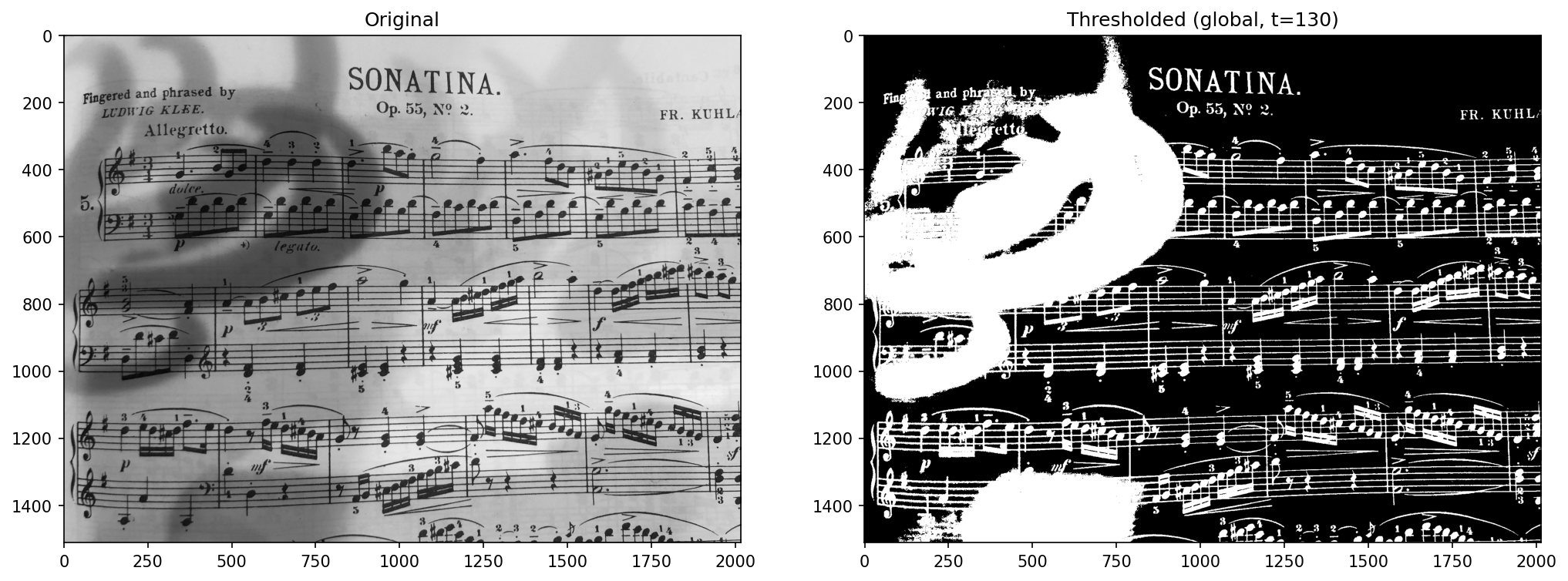
The thresholded result reveals the challenge with global thresholding on unevenly lit documents. The sheet music has a shadow gradient across the page (darker in the upper-left corner). Because we use a single threshold value of 130 for the entire image, the shadowed region is misclassified as "ink" - it produces a large white blob where the shadow was.
Key Takeaway
Global thresholding works well when lighting is uniform, but struggles with shadows and uneven illumination. For real-world document processing, adaptive thresholding (cv2.adaptiveThreshold) computes a local threshold for each pixel neighborhood, making it far more robust to lighting variations.