Image Processing with CV2

A hands-on walkthrough of fundamental image processing operations using OpenCV and Python - covering pixel manipulation, brightness and contrast adjustments, and thresholding techniques.

Prerequisites

This guide uses three libraries that form the backbone of most computer vision work in Python:

import cv2
import numpy as np
import matplotlib.pyplot as plt

• OpenCV (cv2) - the industry-standard library for image processing and computer vision
• NumPy - provides the array data structure that underlies all image representations in OpenCV
• Matplotlib - used here for visualizing images and results

---

Loading and Inspecting an Image

The first step in any image processing pipeline is loading an image and understanding its structure.

image = cv2.imread("Reykjavik-Iceland.jpg")

print("Shape of the image:", image.shape)
print("Top-left pixel [Blue, Green, Red]:", image[0, 0])
print("Data type:", image.dtype)

Shape of the image: (1062, 1600, 3)
Top-left pixel [Blue, Green, Red]: [226 183 134]
Data type: uint8

The .shape attribute returns (height, width, channels). This image is 1062 pixels tall, 1600 pixels wide, and has 3 color channels. Each pixel is stored as a uint8 value (0-255).

The top-left pixel [226, 183, 134] is in BGR order - OpenCV's default channel ordering, not the more common RGB. This is one of the most frequent sources of color bugs when combining OpenCV with other libraries.

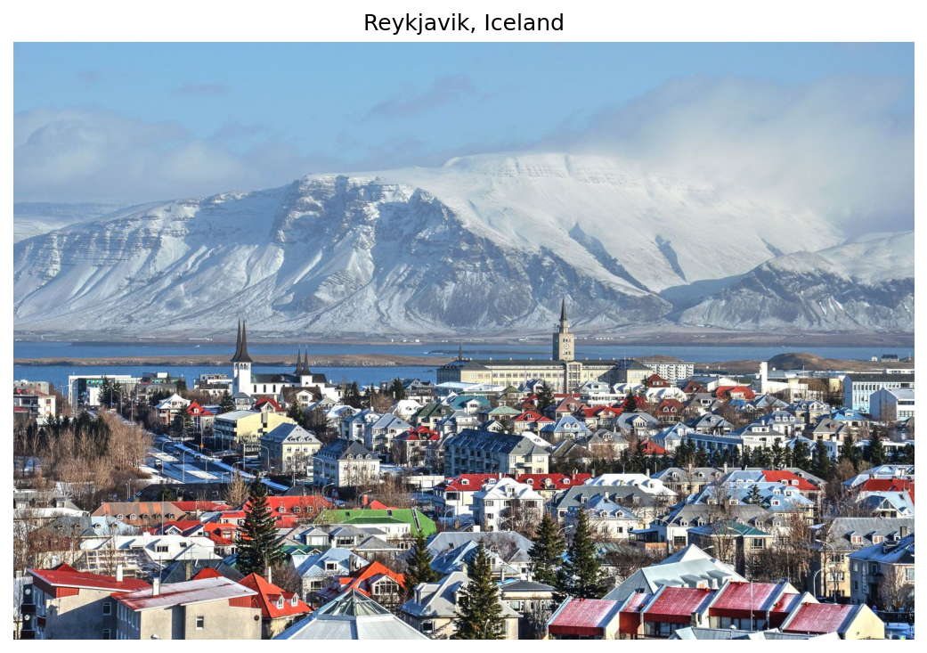
Displaying with Matplotlib

Since Matplotlib expects RGB channel ordering, you need to reverse the channel axis before displaying:

image_rgb = image[:, :, ::-1]

plt.figure(figsize=[8, 5])
plt.imshow(image_rgb)
plt.title("Reykjavik, Iceland")
plt.axis("off")
plt.show()

The slice [:, :, ::-1] reverses the last axis, converting BGR to RGB. Without this conversion, blues and reds would be swapped in the displayed image.

---

Brightness Adjustment

Brightness is controlled by adding or subtracting a constant value from every pixel. OpenCV's cv2.add() and cv2.subtract() handle saturation arithmetic automatically - values are clamped to the 0-255 range instead of wrapping around.

matrix = np.ones(image.shape, dtype="uint8") * 30
img_brighter = cv2.add(image, matrix)
img_darker = cv2.subtract(image, matrix)

The key detail here is the use of cv2.add() and cv2.subtract() instead of Python's + and - operators. NumPy's arithmetic wraps around on overflow (e.g., 255 + 30 becomes 29), which produces ugly artifacts. OpenCV's functions clamp instead: 255 + 30 stays at 255, and 0 - 30 stays at 0.

plt.figure(figsize=[18, 5])
plt.subplot(131); plt.imshow(img_darker[:, :, ::-1]);   plt.title("Darker")
plt.subplot(132); plt.imshow(image_rgb);                 plt.title("Original")
plt.subplot(133); plt.imshow(img_brighter[:, :, ::-1]); plt.title("Brighter")
plt.show()

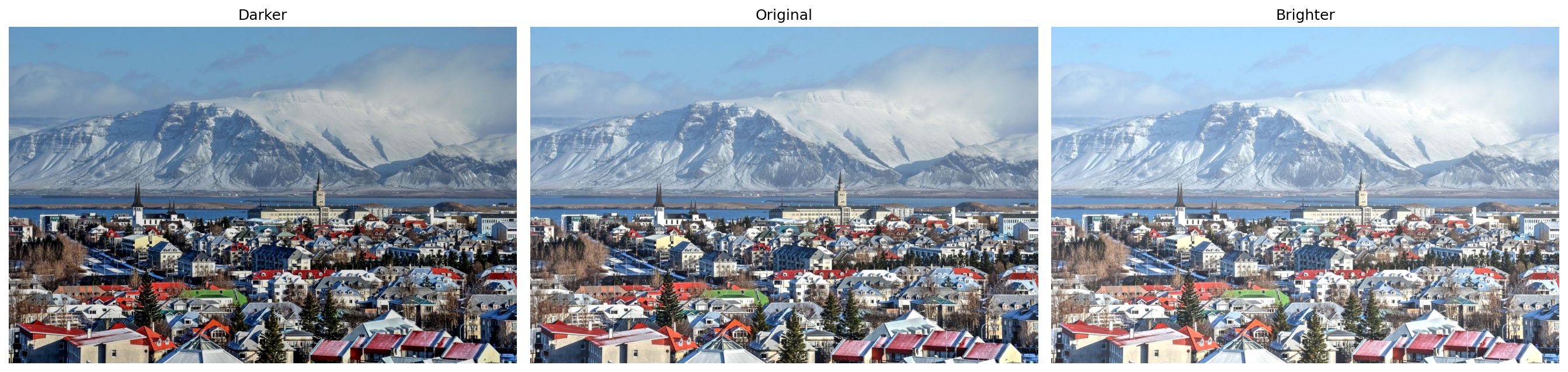
Adding 30 to every pixel shifts the entire histogram to the right (brighter), while subtracting 30 shifts it left (darker). The overall contrast and relative differences between pixels remain unchanged.

---

Contrast Adjustment

Contrast is controlled by multiplying pixel values by a scaling factor. A factor less than 1.0 reduces contrast (compresses the value range), while a factor greater than 1.0 increases contrast (expands the range).

The Wrap-Around Problem

matrix_low = np.ones(image.shape) * 0.8
matrix_high = np.ones(image.shape) * 1.2

img_lower = np.uint8(cv2.multiply(np.float64(image), matrix_low))
img_higher = np.uint8(cv2.multiply(np.float64(image), matrix_high))

The multiplication is done in float64 to avoid overflow during computation. However, casting back to uint8 with np.uint8() uses modular arithmetic - a pixel value of 280 wraps to 280 - 256 = 24, turning bright areas unexpectedly dark.

plt.figure(figsize=[18, 5])
plt.subplot(131); plt.imshow(img_lower[:, :, ::-1]);  plt.title("Lower Contrast")
plt.subplot(132); plt.imshow(image_rgb);               plt.title("Original")
plt.subplot(133); plt.imshow(img_higher[:, :, ::-1]); plt.title("Higher Contrast (wrap)")
plt.show()

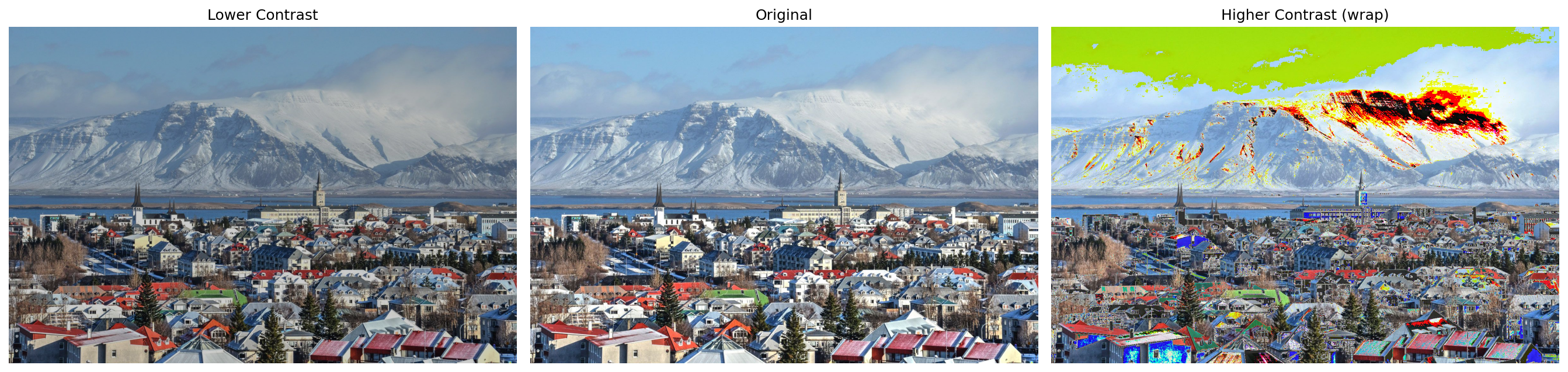
Notice the wrap-around artifacts in the "Higher Contrast" image - bright regions that overflowed past 255 wrapped back to low values, creating dark splotches in areas that should be the brightest.

The Fix: Clipping

The correct approach is to clip values to the valid range before casting:

img_higher_clipped = np.uint8(np.clip(
    cv2.multiply(np.float64(image), matrix_high), 0, 255
))

np.clip() caps all values at 255 (and floors at 0), preventing the wrap-around. Bright pixels that exceed 255 are simply set to 255 - they lose detail, but the result looks natural rather than corrupted.

plt.figure(figsize=[18, 5])
plt.subplot(131); plt.imshow(img_lower[:, :, ::-1]);          plt.title("Lower Contrast")
plt.subplot(132); plt.imshow(image_rgb);                       plt.title("Original")
plt.subplot(133); plt.imshow(img_higher_clipped[:, :, ::-1]); plt.title("Higher Contrast (clipped)")
plt.show()

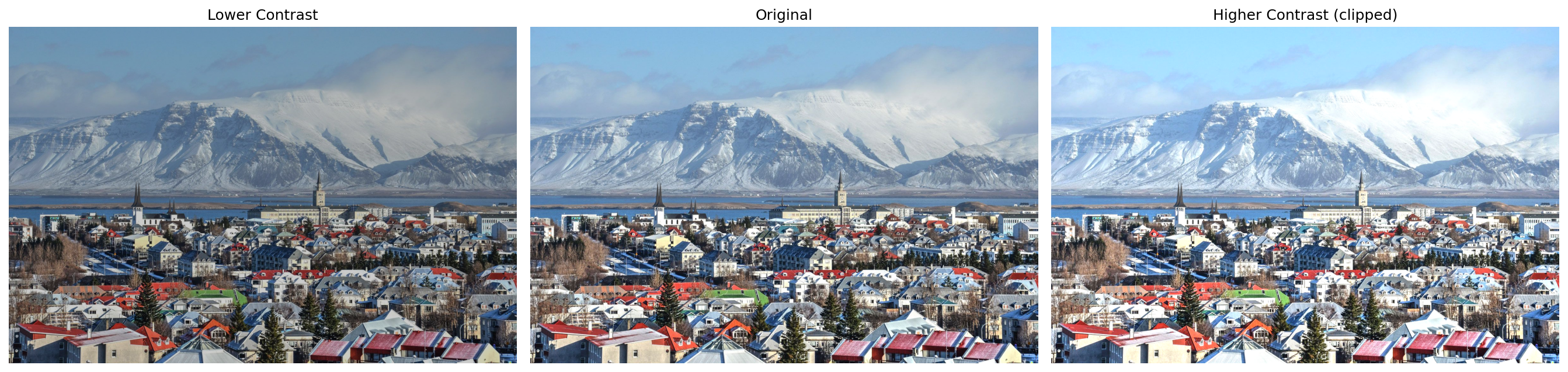
The clipped version preserves the intended brightening effect without the ugly wrap-around artifacts.

---

Thresholding

Thresholding converts a grayscale image into a binary (black and white) image by applying a simple rule: pixels above a threshold become white (255), and pixels below become black (0). It is one of the most fundamental segmentation techniques.

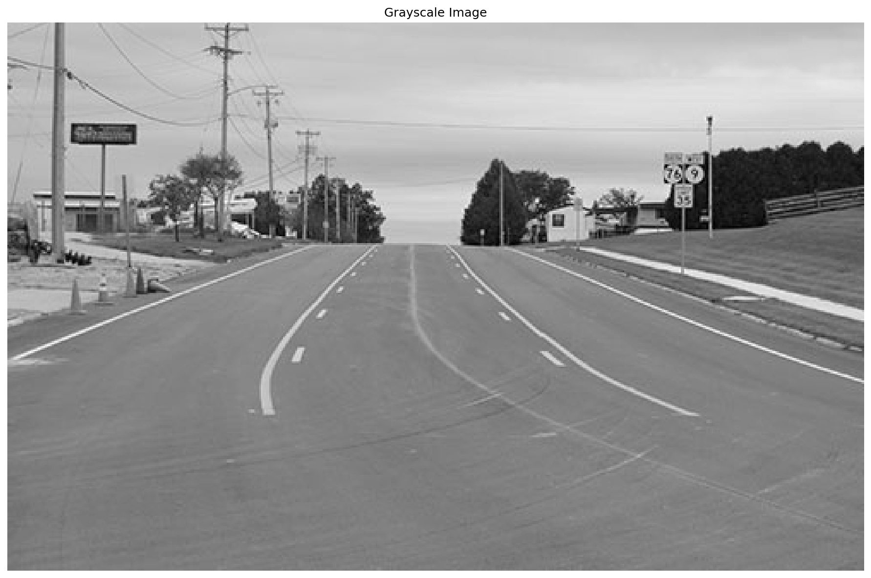
Loading a Grayscale Image

img_lanes = cv2.imread("lanes_tesla.jpg", cv2.IMREAD_GRAYSCALE)

The cv2.IMREAD_GRAYSCALE flag tells OpenCV to convert the image to a single channel during loading, rather than loading as BGR and converting afterward.

plt.figure(figsize=[16, 8])
plt.imshow(img_lanes, cmap="gray")
plt.title("Grayscale Image")
plt.axis("off")
plt.show()

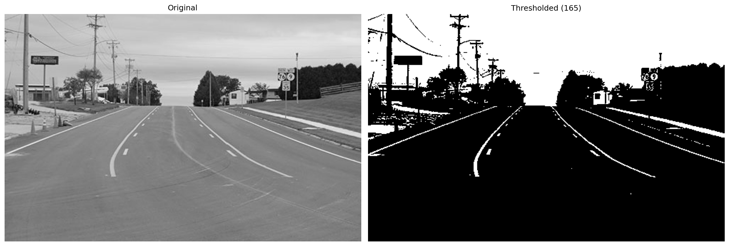
Applying a Binary Threshold

_, img_thresh = cv2.threshold(img_lanes, 165, 255, cv2.THRESH_BINARY)

cv2.threshold() returns two values: the threshold used (which we discard with _) and the output image. Every pixel brighter than 165 becomes 255 (white); everything else becomes 0 (black).

plt.figure(figsize=[16, 8])
plt.subplot(121); plt.imshow(img_lanes, cmap="gray");  plt.title("Original")
plt.subplot(122); plt.imshow(img_thresh, cmap="gray"); plt.title("Thresholded (165)")
plt.show()

Choosing the Right Threshold

The threshold value dramatically affects what gets extracted from the image. Too low and you capture noise; too high and you lose important features.

_, thresh_100 = cv2.threshold(img_lanes, 100, 255, cv2.THRESH_BINARY)
_, thresh_165 = cv2.threshold(img_lanes, 165, 255, cv2.THRESH_BINARY)
_, thresh_200 = cv2.threshold(img_lanes, 200, 255, cv2.THRESH_BINARY)

plt.figure(figsize=[20, 5])
plt.subplot(131); plt.imshow(thresh_100, cmap="gray"); plt.title("Threshold = 100")
plt.subplot(132); plt.imshow(thresh_165, cmap="gray"); plt.title("Threshold = 165")
plt.subplot(133); plt.imshow(thresh_200, cmap="gray"); plt.title("Threshold = 200")
plt.show()

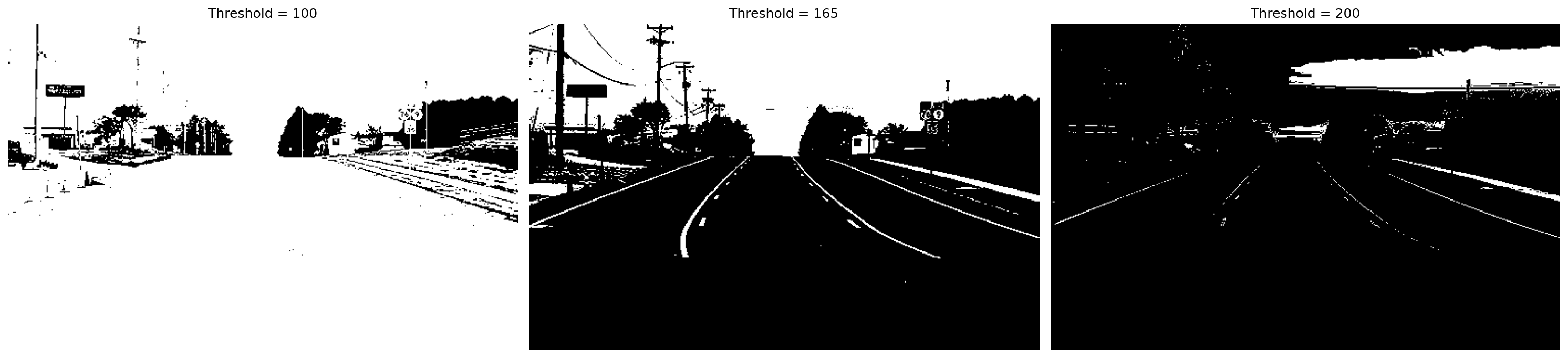
• Threshold = 100 - captures too much of the scene, including road surface and sky
• Threshold = 165 - a reasonable balance that isolates lane markings and bright features
• Threshold = 200 - very aggressive, only the brightest pixels survive

There is no universally correct threshold - it depends entirely on the image content and what you are trying to extract.

---

Global vs. Adaptive Thresholding

Global thresholding applies the same cutoff to the entire image. This works well when lighting is uniform, but fails when the image has varying illumination - a common problem in real-world photos.

Adaptive thresholding solves this by computing a different threshold for each pixel based on its local neighborhood.

img_coins = cv2.imread("coins.jpg", cv2.IMREAD_GRAYSCALE)

_, coins_thresh_50 = cv2.threshold(img_coins, 50, 255, cv2.THRESH_BINARY)
_, coins_thresh_130 = cv2.threshold(img_coins, 130, 255, cv2.THRESH_BINARY)
coins_thresh_adp = cv2.adaptiveThreshold(
    img_coins, 255, cv2.ADAPTIVE_THRESH_MEAN_C, cv2.THRESH_BINARY, 13, 7
)

The cv2.adaptiveThreshold() parameters:

• 255 - the value assigned to pixels that pass the threshold
• cv2.ADAPTIVE_THRESH_MEAN_C - the threshold for each pixel is the mean of its neighborhood minus a constant
• cv2.THRESH_BINARY - output is binary (0 or 255)
• 13 - the size of the neighborhood window (13x13 pixels)
• 7 - the constant subtracted from the neighborhood mean

plt.figure(figsize=[10, 8])
plt.subplot(221); plt.imshow(img_coins, cmap="gray");        plt.title("Original")
plt.subplot(222); plt.imshow(coins_thresh_50, cmap="gray");  plt.title("Thresholded (global: 50)")
plt.subplot(223); plt.imshow(coins_thresh_130, cmap="gray"); plt.title("Thresholded (global: 130)")
plt.subplot(224); plt.imshow(coins_thresh_adp, cmap="gray"); plt.title("Thresholded (adaptive)")
plt.show()

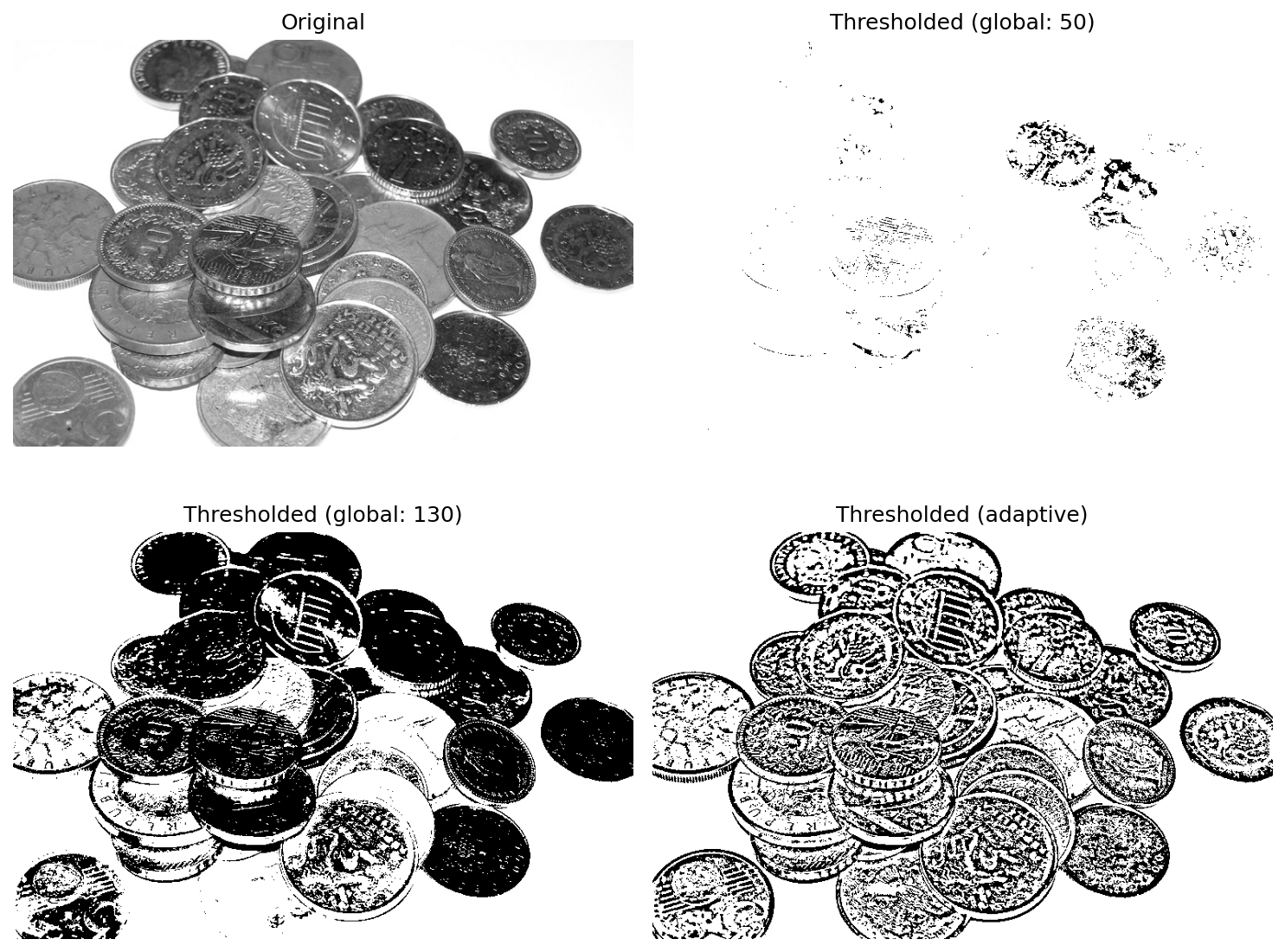
The results illustrate the limitations of global thresholding:

• Global at 50 - too permissive, most of the image is white
• Global at 130 - better, but coins in darker regions are lost while coins in brighter regions are overexposed
• Adaptive - handles the uneven lighting gracefully, producing clean coin outlines across the entire image regardless of local brightness

Adaptive thresholding is the preferred approach whenever lighting conditions vary across the image, which is the norm in most practical applications.

---

Key Takeaways

1. OpenCV loads images in BGR order - always convert to RGB before displaying with Matplotlib or passing to other libraries
2. Use cv2.add() / cv2.subtract() for brightness adjustments - they handle saturation correctly, unlike raw NumPy arithmetic
3. When adjusting contrast via multiplication, always clip values with np.clip() before casting to uint8 to avoid wrap-around artifacts
4. Thresholding is a powerful but simple segmentation tool - the threshold value must be tuned to the specific image and task
5. Adaptive thresholding outperforms global thresholding in scenes with uneven illumination, making it more robust for real-world applications

Further Reading

• OpenCV Thresholding Tutorial
• OpenCV Image Arithmetic
• NumPy Array Manipulation