NLP Introduction

Natural Language Processing techniques and patterns for building text-understanding systems at Enddesk.

Prerequisites

The code snippets on this page require several Python libraries. Install them all at once with:

pip install scikit-learn sentence-transformers numpy spacy transformers torch

Or download the requirements.txt and run:

pip install -r requirements.txt

The Named Entity Recognition section also needs a spaCy language model:

python -m spacy download en_core_web_sm

What Is NLP and Why Does It Matter?

Every day, humans produce enormous amounts of text: emails, social media posts, voice transcripts, chat messages, reviews. According to Research Solutions, over 80% of the data we generate is unstructured language. NLP is the branch of artificial intelligence dedicated to giving machines the ability to read, interpret, and respond to all of that human language in a useful way.

At its core, NLP sits at the intersection of linguistics and computer science. It acts as a translator between the messy, nuanced way people communicate and the rigid, numerical world that computers operate in. Without NLP, a computer sees a sentence like "I loved that restaurant" as nothing more than a sequence of characters; with NLP, it can recognize the positive sentiment, identify "restaurant" as an entity, and even infer that you might want similar recommendations.

Why Language Is Exceptionally Hard for Computers

Human language is full of traps that we navigate effortlessly but that trip up machines constantly:

• Ambiguity - A sentence like "I saw her duck" has at least two valid readings: witnessing a bird or watching someone dodge. Humans resolve this instantly from context; algorithms need explicit strategies to do the same.
• Polysemy - The word "bank" can mean a financial institution or the edge of a river. Multiply this by thousands of common words and you get a sense of the scale of the problem (Polysemy - Evidence from Linguistics and Contextualized Language Models).
• Sarcasm and tone - When someone writes "Oh great, another meeting," the literal words are positive, but the meaning is the opposite. Detecting this requires understanding intent, which remains one of the hardest open problems in the field.

How NLP Got Here: From Handwritten Rules to Learned Patterns

The field has gone through a dramatic transformation over the past seven decades (Digital RGS - The Evolution of NLP):

1. Rule-based era (1950s-1990s) - Early systems like ELIZA relied on manually crafted if-then patterns. They worked in narrow, controlled scenarios but broke down the moment language got creative or unpredictable.
2. Statistical era (1990s-2010s) - Researchers shifted to probability: instead of telling a machine what language is, they showed it millions of examples and let it learn patterns. Techniques like Hidden Markov Models and n-grams powered the first generation of spam filters and machine translators.
3. Deep learning and transformers (2010s-present) - Neural networks, and especially the transformer architecture introduced in the landmark "Attention Is All You Need" paper (video explainer), changed everything. Models like BERT and GPT can now grasp context across entire documents, enabling applications from conversational AI to code generation.

The Basic NLP Pipeline

Before any model can work with text, the raw input needs to be cleaned and converted into a numerical form the computer can process. A typical pipeline looks like this:

import re
from typing import List
from sklearn.feature_extraction.text import CountVectorizer

def clean_and_tokenize(text: str) -> List[str]:
    text = text.lower()
    text = re.sub(r"[^a-z0-9\s]", "", text)
    tokens = text.split()
    stop_words = {"the", "a", "an", "is", "in", "on", "at", "to", "for"}
    return [t for t in tokens if t not in stop_words]

raw = "NLP is Amazing - let's explore it!"
tokens = clean_and_tokenize(raw)  # ['nlp', 'amazing', 'lets', 'explore', 'it']

vectorizer = CountVectorizer()
X = vectorizer.fit_transform([" ".join(tokens)])
print(dict(zip(vectorizer.get_feature_names_out(), X.toarray()[0])))

The steps are straightforward: lowercase everything so "NLP" and "nlp" are treated as the same token, strip out punctuation and special characters, split into individual words (tokenization), drop common filler words that carry little meaning, and finally convert the remaining tokens into numbers, because at the end of the day, computers do not read; they calculate.

What Does a Vectorized Result Actually Look Like?

Once the text passes through the CountVectorizer, each unique word gets a count. For our example sentence the output is a dictionary mapping every token to how many times it appeared:

{
  'amazing': np.int64(1),
  'explore': np.int64(1),
  'it': np.int64(1),
  'lets': np.int64(1),
  'nlp': np.int64(1)
}

Visually, you can think of it as a bar chart where every word has a frequency of one:

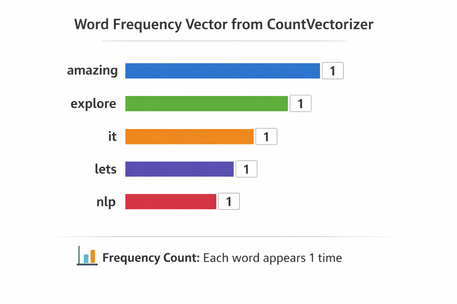
But the computer does not see labels or colored bars. What it actually stores is a flat numeric array one slot per word, ordered alphabetically:

Vector: [1, 1, 1, 1, 1]
Index:   0  1  2  3  4

Each position maps to a word: index 0 → amazing, index 1 → explore, and so on. This is the representation the model works with.

From Vector to Prediction

Having numbers is only half the story. A machine learning model assigns a weight to every word based on what it learned during training. If the model was trained on labeled reviews, it might discover that "amazing" almost always appears in positive text, so it gives that word a strong positive weight. A simplified scoring formula looks like this:

score = (amazing × +2) + (bad × −2) + (dont × −1.5) + …

For our sentence, "amazing" is present (value 1) and carries a weight of +2, while words like "bad" are absent (value 0), contributing nothing. The final score skews positive, and the model classifies the text accordingly. This is the core loop behind text classification: vectorize the words, multiply by learned weights, and let the total score drive the decision.

Embeddings & Semantic Search

CountVectorizer turns words into simple frequency counts, but it has no idea that "training" and "fine-tune" mean something similar. Embedding models solve this by converting entire sentences into dense numeric vectors where meaning is preserved sentences that talk about similar things end up close together in vector space.

from sentence_transformers import SentenceTransformer
import numpy as np

model = SentenceTransformer("all-MiniLM-L6-v2")

documents = [
    "How to fine-tune a language model",
    "Best practices for prompt engineering",
    "Deploying ML models to production",
]

embeddings = model.encode(documents)

query = "training a custom LLM"
query_embedding = model.encode([query])

similarities = np.dot(embeddings, query_embedding.T).flatten()
best_match = documents[np.argmax(similarities)]

print(f"Best match: {best_match}")
print(f"Similarity: {np.max(similarities)}")

# Best match: Deploying ML models to production
# Similarity: 0.3749297857284546

The Embedding Database

When you call model.encode(documents), the model reads each sentence and compresses its meaning into a fixed length array of 384 floating-point numbers. This is because SentenceTransformer("all-MiniLM-L6-v2") is a pretrained model with a fixed embedding size of 384 dimensions. The result is a matrix, one row per document:

embeddings = model.encode(documents)

# array([[ 0.04902101, -0.0577189 ,  0.03843281, ...,  0.05040744,
#         -0.0075976 , -0.02286296],
#        [ 0.01633435,  0.0421459 ,  0.02429694, ...,  0.11636557,
#         -0.02745431,  0.03348003],
#        [ 0.02428063, -0.13008808,  0.01858209, ..., -0.06775104,
#          0.06105504, -0.04895689]], shape=(3, 384), dtype=float32)

Three documents, each represented by 384 numbers. You can think of each row as a coordinate in a 384 dimensional space. Documents with similar meaning land near each other in that space:

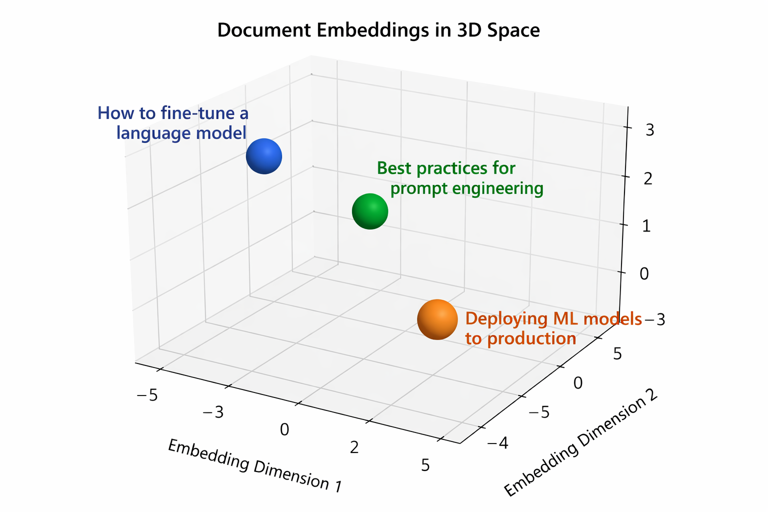
The chart above shows a simplified 3D projection of those 384 dimensional vectors. In reality the space has far more dimensions, but the idea is the same: related documents cluster together.

The Query Vector

The query goes through the exact same process. model.encode([query]) produces a single row with the same 384 dimensions:

query_embedding = model.encode(["training a custom LLM"])

# array([[ 2.32793093e-02, -4.95579652e-02, -2.85389065e-03,
#          .....
#         -3.47590260e-02, -1.13572009e-01, -3.70876007e-02]], dtype=float32)

One query, one vector. Same shape as each document row, so we can directly compare them.

Computing Similarity

The dot product is the formula behind the comparison. It multiplies matching positions and sums everything:

dot(A, B) = A₁ × B₁ + A₂ × B₂ + ... + Aₙ × Bₙ

A simple 2D example makes this concrete:

doc   = [1, 2]
query = [3, 4]

(1 × 3) + (2 × 4) = 3 + 8 = 11

The higher the result, the more aligned the two vectors are. With 384 dimensions instead of 2, the math is identical, just more multiplications to sum up.

np.dot(embeddings, query_embedding.T).flatten() applies this formula between the query vector and every document vector. The higher the score, the closer the meaning:

similarities = np.dot(embeddings, query_embedding.T).flatten()

# array([0.220232  , 0.27529132, 0.3749298 ], dtype=float32)
# similarities = [score_doc1, score_doc2, score_doc3]

Document 3 ("Deploying ML models to production") scores highest at 0.375, followed by document 2 ("Best practices for prompt engineering") at 0.275, and document 1 ("How to fine-tune a language model") at 0.220. So np.argmax picks document 3:

best_match = documents[np.argmax(similarities)]
# 'Deploying ML models to production'

Even though the query "training a custom LLM" shares no exact words with the best match, the embedding model understands the semantic overlap, both are about putting ML models to work.

Named Entity Recognition (NER)

Extract structured information from unstructured text:

import spacy

nlp = spacy.load("en_core_web_sm")
doc = nlp("Enddesk launched a new AI product in San Francisco on March 2026.")

for ent in doc.ents:
    print(f"{ent.text} -> {ent.label_}")

# Enddesk -> ORG
# San Francisco -> GPE
# March 2026 -> DATE

spaCy is a fast, production-ready NLP library in Python used to process and understand text. You can get a lot out of this library, including NER which is what we used it for in this example. Here is what spaCy can extract from text:

• Tokens - individual words and punctuation
• Part-of-speech - noun, verb, adjective, etc.
• Named entities (NER) - people, organizations, locations, dates
• Dependencies - sentence structure and how words relate to each other

spaCy vs Transformers

spaCy and Transformers (covered in the next section) take different approaches. spaCy is optimized for speed and production pipelines, while Transformers trade speed for deeper language understanding:

Feature	spaCy	Transformers
Speed	Very fast	Slower
Accuracy	Good	Very high
Ease of use	Easy	Easy (with pipeline)
Deep understanding	Limited	Advanced
Production use	Excellent	Heavier

For tasks like NER where speed matters and the built-in models are accurate enough, spaCy is a great choice. When you need higher accuracy or more nuanced understanding, Transformers are worth the extra cost.

Text Classification with Transformers

Transformers answer a simple question: "How does this text feel?" This is sentiment analysis, giving the model a piece of text and getting back an opinion: positive, negative, or somewhere in between.

In this example we use the high level pipeline API from Hugging Face Transformers. This API hides all the complex machine learning steps behind a single function call:

from transformers import pipeline

classifier = pipeline(
    "text-classification",
    model="distilbert-base-uncased-finetuned-sst-2-english",
)

result = classifier("This product is absolutely fantastic!")

# [{'label': 'POSITIVE', 'score': 0.9998809099197388}]

When you call pipeline(...), three things happen under the hood:

1. A tokenizer loads: it splits your text into tokens the model can understand
2. A model loads: in this case DistilBERT, a smaller and faster version of BERT
3. Pretrained weights load: the model already comes trained on sentiment data, so you do not need to train anything yourself

This specific model was trained on the SST-2 dataset (Stanford Sentiment Treebank), which consists of movie reviews labeled as positive or negative. That is why it is so confident about "This product is absolutely fantastic!", it has seen thousands of similar phrases during training.

The result you get back has two fields:

• label: the predicted class (POSITIVE or NEGATIVE)
• score: the confidence level, ranging from 0 to 1 (0.999 means the model is 99.9% sure)

What Else Can the Pipeline API Do?

Text classification is just one of many tasks the pipeline API supports. You can swap out the task name and get a completely different capability:

Task	Pipeline name	What it does
Sentiment analysis	text-classification	Classifies text as positive, negative, etc.
Named entity recognition	ner	Extracts people, places, organizations from text
Question answering	question-answering	Answers a question given a context paragraph
Text summarization	summarization	Condenses long text into a shorter version
Translation	translation	Translates text between languages
Text generation	text-generation	Generates text from a prompt
Fill in the blank	fill-mask	Predicts missing words in a sentence
Zero-shot classification	zero-shot-classification	Classifies text into custom labels without training
Token classification	token-classification	Labels individual tokens (POS tagging, chunking)
Feature extraction	feature-extraction	Produces embeddings for downstream tasks
Conversational	conversational	Multi-turn chatbot dialogue
Image classification	image-classification	Classifies images into categories
Object detection	object-detection	Detects and locates objects in images
Automatic speech recognition	automatic-speech-recognition	Converts audio to text

Every one of these follows the same pattern: pick a task, pick a model, and call the pipeline. The API handles tokenization, inference, and post processing for you.

Key Takeaways

1. NLP bridges the gap between how humans communicate and how machines compute
2. Language is hard for computers because of ambiguity, polysemy, and context-dependence
3. The field evolved from brittle hand-coded rules to flexible, data-driven models
4. Every NLP workflow starts with cleaning and vectorizing text
5. Embeddings unlock powerful semantic search and clustering
6. Use pretrained models and fine-tune for your domain
7. Evaluate NLP systems with task-specific metrics (F1, BLEU, ROUGE)